Confidence Interval
From Central Limit Theorem, we learned that the mean of the sampling distribution is very close to the population mean and standard deviation is equal to the population standard deviation divided by square root of sample size.
Advancing this one step further, if we were to choose any one sample of size 'n' and compute the mean, how confident we are that it will be true population mean? The answer is given by 'Confidence Interval' concept. We can never be sure that one single value will equal the population mean. But, we can compute an interval which contains the true population mean with some confidence. We can never be 100% sure that the population mean will lie in the interval and also it is not necessary to do so. Therefore, we compute the intervals with varying confidence requirements, such as 90%, 95%, 99%.
We know from our normal distribution discussion that we contain 95% of the data when we contain 1.96 times the standard deviation on either side of the mean. Using this knowledge, we compute our 95% confidence interval for sample mean that will contain the true population mean as interval with 1.96σx¯ on either side of the mean.
We don't know where in the interval µ is but we can say that we are 95% confident that the interval contains the µ or in other words, there is a 5% chance that the interval does not contain the population mean µ.
We can compute the mean and standard deviation from the sample but we need
to also determine the accuracy for it to be useful. We can choose any high margin of error such as 90%, 95% and 99%
to estimate the true population mean µ by attaching this error to the computed mean x¯ from the
sample.
We denote the error by the symbol α, so 90% margin translates to α=(1-0.90)=0.10.
To find 95% error margin, we find the zα/2=z0.025
We use the normal distribution table to find the area to the right of zα/2.
Following summarizes the values needed:
| 1-α | 0.80 | 0.85 | 0.90 | 0.95 | 0.99 |
|---|---|---|---|---|---|
| zα/2 | 1.28 | 1.44 | 1.645 | 1.96 | 2.58 |
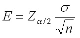
where, E = error permitted or desired.
Therefore our confidence interval is:
x¯+/-E
Sample Size
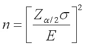
Yet, another useful way to look at the above theory is to find the quantity of samples required to be (1-α)% confident that the error in our estimation of true mean µ won't exceed E on either side i.e. +/- E. The following equation defines the above concept:
Example:
A water supply reservoir is being tested for estimating average suspended solids per unit volume of water.
From past studies, it is know that the standard deviation σ = 30 ppm. How many samples are needed to be
95% confident that the error in estimating the average won't exceed 5 ppm?
Solution:
Here we need a confidence of 95%. Therefore our α is 0.05.We find that our Zα/2 or Z0.025 is 1.96. Our permitted error is E = 5 ppm. i.e., The tested value could be +/- 5 ppm from true mean(with 95% confidence only !). Therefore the number of samples required can be calculated using the formula above as n = 139.
In simple language, if we repeat our experiment of 139 tests several times and compute the confidence intervals, then 95% of those confidence intervals will contain the true µ.
If sample size is large, we can replace the µ with x¯ and σ with s.
